
Historically, there have been three main use cases for WURFL and, more generally, Device Detection:
- (Mobile) Web Optimization: using WURFL to serve a customized user-experience to different classes of devices.
- Ad Tech: relying on device capabilities as one of the factors to pick relevant ads for end-users.
- Analytics: augment your data with WURFL to slice and dice your log data and get deeper insight into how users utilize your service,
This blog post illustrates a concrete scenario. We explore how you can use WURFL to discover new correlations in data, and ultimately leverage Machine Learning (ML) techniques to create regression models and classifiers. This approach may allow organizations to make predictions about user behavior thanks to WURFL.
Important Note: This article assumes that the reader is familiar with Machine Learning concepts, as well as tools such as Jupyter Notebook, Python, Pandas and Seaborn. Wherever possible, we will provide hints that will allow “lay” readers to get the gist of what is going on.
While introducing Machine Learning is outside the scope of this article, the article may still provide interesting reading to those who want to understand more about a vast new field at the intersection of statistics, programming and data science.
Our Scenario
A pretty common scenario in Ad Tech these days is Real-Time Bidding (RTB). As a user visits a website (on their phones, laptop, tablet, Smart TV or wristwatch), the Ad Tech ecosystem will run a fully-fledged real-time auction for each page request. Advertisers, or someone acting on their behalf, can bid on those impressions. The bid-winner gets the right to display their ad to the user.
Quoting Wikipedia:
“Real-time bidding (RTB) is a means by which advertising inventory is bought and sold on a per-impression basis, via instantaneous programmatic auction, similar to financial markets. With real-time bidding, advertising buyers bid on an impression and, if the bid is won, the buyer’s ad is instantly displayed on the publisher’s site. Real-time bidding lets advertisers manage and optimize ads from multiple ad-networks, allowing them to create and launch advertising campaigns, prioritize networks, and allocate percentages of unsold inventory, known as backfill.
Real-time bidding is distinguishable from static auctions by how it is a per-impression way of bidding, whereas static auctions are groups of up to several thousand impressions. RTB is promoted as being more effective than static auctions for both advertisers and publishers in terms of advertising inventory sold, though the results vary by execution and local conditions. RTB replaced the traditional model.”
In this context, it only makes sense that advertisers will try to squeeze the last bit of information out of those HTTP headers, trying to determine whether a certain user is worth, say, a 15 cents bet to show them a banner ad.
Artificial Intelligence (and more specifically Machine Learning) can play an important role in this area. For example, a ML regression or classification may establish a correlation between HTTP Request headers and a user’s propensity to click on our banner ad. A “high-propensity” request is probably the one we want to bid on.
Note: you may be familiar with the differences between Artificial Intelligence, Machine Learning and Deep Learning. If not, the schema below may come handy.

For the purpose of these tutorials, we have obtained a dataset [LINK] that contains HTTP requests from a variety of browsers and devices, ranging from desktop web browser, to smartphones, to tablets and SmartTVs. For each request, an additional field called ‘Platform-User-Click’ tells us whether the end-user has clicked on our banner ad (BA) or not.
We can analyze this dataset to find what correlations exist between HTTP headers and a user’s willingness to click on the BA.
Of course, as you probably already know, people are no longer easily convinced to click on ads these days, hence we cannot expect a super obvious correlation between an HTTP Client (as represented by the User-Agent string and other headers) and the actual click.
Yet, we suspect that some correlations do exist and that we can exploit certain “features” to estimate user propensity to engage with our banner ad (we put the term “feature” in quotes as we are using it sort of ambiguously to refer to actual device features according to Device Detection speech, but also hinting at the use of the same term in the context of regressions models and classifiers, i.e. the Machine Learning domain).
Initially, we will explore our dataset and try to discover properties and correlations without the help of WURFL. At a later stage, we will augment our data set with WURFL capabilities to determine how we can achieve greater insight thanks to Device Detection.
Note: we are going to use Jupyter Notebook for our data exploration. This is pretty much a de-facto standard among many data scientists (particularly those who picked Python as their language of choice). If you are not familiar with it, check it out.
This 15M data.json.gz [ADD LINK TO DOWNLOADABLE DATASET] contains one million HTTP requests in JSON format, without any added WURFL capabilities.
$ ls -la data.json.gz
-rwxrwxrwx 1 passani passani 16225458 Feb 24 21:48 data.json.gz
In addition to the HTTP headers, ‘Platform-User-Click’ tells us whether the user has clicked on the ad for this particular request.

Let’s load the data into a Pandas DataFrame.
Note: if you don’t know what Pandas is, think Microsoft Excel for data scientists: there is no UI, but all the data, in much larger amounts than an Excel spreadsheet can usually manage, is kept in memory; data scientists can slice and dice the data both programmatically and through an interactive environment such as Jupyter Notebook (arguably, Jupyter Notebook is the Pandas UI).
Let’s kick it by parsing our JSON file:

Now it’s in a Pandas dataframe. Let’s take a look:

All fields are loaded. Unsurprisingly, many fields are very sparsely populated (certain HTTP headers are specific to side-loaded browsers such as Opera Mini and UCBrowser):
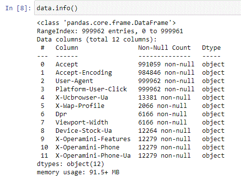
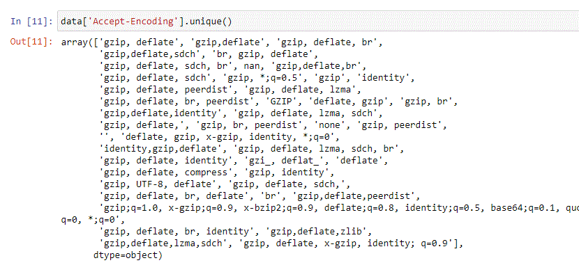
Accept and Accept-Encoding columns have non-null values 99% of the times. A closer look at those values, though, reveals that they have high variance and are not very useful.
Note: Variance is a fundamental concept in statistics and hence an important one in Machine Learning. Hard to explain what it is without getting totally side-tracked. Let’s say that you want your model to “mimic your data” or it won’t be very good at predicting, that’s why you want low variance. On the other hand, you want to avoid the mistake of mimicking your data too closely or you may find yourself with a model that mimics your data very well, while doing a lousy job on new data. This is called “overfitting” and you want to avoid that. For an intro to variance and the plague of overfitting, this article might provide a good start.
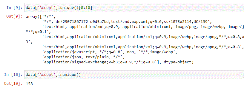
Looking at the values, they would not be particularly valuable to build a model.
Let’s look at the User-Agent:
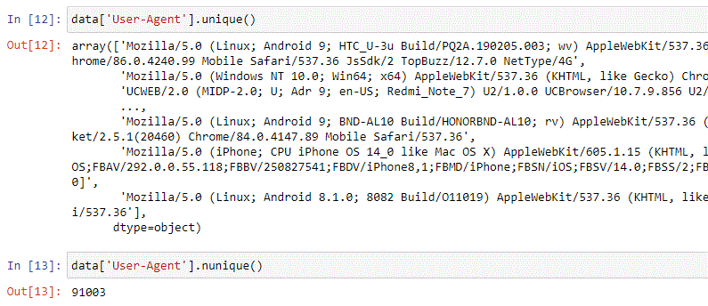
The User-Agent column has lots of valuable information, as we know. Given the form it comes in, though, we cannot easily extract structured information (such as make, model, browser, OS, etc.) from it (Spoiler: you actually can with WURFL. Stay tuned)
Let’s take a look at our target class Platform-User-Click:

Only a little more than 1% of our data refers to an actual click. This is what data scientists call a highly imbalanced dataset: people will click on ads pretty rarely these days.
Imbalanced datasets are not a rarity, but they certainly pose additional challenges for those who only have limited experience as data scientists. Some ML applications are about building predictions that “trigger” in just a tiny fraction of situations. Think of Credit Card fraud, for example. Out of one million transactions, only a few hundred (i.e. 0.01% or less) are fraudulent. Alternatively, for a different example, imagine building a classifier that tries to determine wherever someone going through security at an airport is a terrorist. In those cases, the situations we want to “flag” are just a handful out of tens of millions of travelers that show up at airports each year.
After we have verified that we cannot find much correlation between our UA strings and a user’s propensity to click on our banners, let’s enrich our data with WURFL Device Detection and start exploring again.
Note: we have separated our data into three Jupyter Notebooks. At the end of each notebook we have saved the data into a compressed dataset that can be used as the starting point for the next one:

Enter WURFL
We would like to use a couple of standard ML/AI techniques to verify that there is not much correlation between UA strings and users’ decisions to click.
The User-Agent string is the most informative column available but cardinality is very high so it would be very expensive to train the model based on those values. And that’s not the only issue.
First our training data would be very sparse in spite of the fact that we have one million records.
Secondly, those familiar with Device Detection will know that User-Agents are “a moving target”. The User-Agent associated with a new popular device today is going to refer to a second-hand old device two years from now, i.e. our model’s performance might “deteriorate” pretty quickly as newer devices enter the market. We may want to keep this in mind.
These are issues that we need to address as we explore strategies to create our model.
Let’s augment our dataset with additional device data from WURFL. This is what we are going to show you in the next notebook:
IMPORTANT NOTE: DO NOT TRY TO INSTALL PyWURFL with: #!pip install pywurfl Please obtain PyWURFL from ScientiaMobile and install it following the instruction provided from your customer vault. There is a conflict with a legacy PyWURFL module (outside of ScientiaMobile’s control) that, if installed by mistake, should first be uninstalled for successful install of pywurfl
Let’s first load pywurfl and prepare the static capabilities and virtual capabilities (vCaps) that we plan to explore:
Note: you’ll need to refer to the WURFL capabilities documentation to discover which ones are static and which ones are virtual. Under the hood, virtual capabilities are calculated at run-time, while regular capabilities are not. As calculating vCaps can be an expensive operation, API users need to be aware of which capabilities are virtual and which are static.
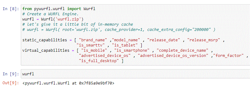
The WURFLwurfl object has been created. Let’s check that everything is in place by loading a single device, its corresponding capabilities and the list of capability names (this list will be handy later to initialize the names of the new columns in the new augmented dataframe):

Everything looks good. We are now ready to go for the real thing. We will build a mock HTTP request out of the headers in each record and feed it to the WURFL Python API to obtain the values of all the new features.
Note: While the User-Agent string is the most important HTTP header by far (as far as Device Detection goes), passing all headers to the WURFL API is the most future-proof way to use it. Also this is a time consuming process, albeit the actual time greatly depends on your hardware and memory.
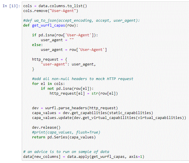
Let’s see what we got:

Let’s explore and find whether there are obvious associations, starting with the device MSRP price. The following dataViz will tell us how the price of devices is “distributed” in our dataset:

Let’s also take a look at brands:

How do price and brand correlate? Unsurprisingly, Apple is sort of pricey.
Let’s explore if price makes a difference once we break down our data by brand.
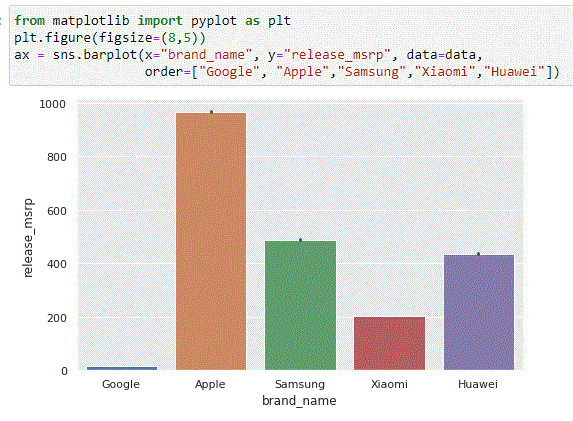
There appears to be a correlation between the device price and user propensity to click on a banner ad.

There also seems to be a correlation between newer OSes and a user’s tendency to click on a banner ad.
Note: you may have noted those tiny black lines at the top of each bar. Data scientists and those versed in statistics will immediately recognize Confidence Intervals, i.e. since the value is an average, the line gives you an indication of where 95% of the values for that category are distributed. For a better understanding of Confidence Intervals and Bootstrapping, this good video should do.
Let’s create a new OS_and_Ver column that will merge OS and respective versions into one single string. This will help us visualize.

Let us delve a little deeper into the release date. The capability value can be broken down into separate month and year columns.
If you are familiar with Pandas, not much explanation is needed for the following line, with the possible exception of expand=True to get the result of split in the form of columns (a Dataframe).

Let’s order our data by year and order it by frequency of ‘1’s.
Note: if you are not familiar with crosstab (cross tabulation) in Pandas, you may want to take a look at this video.

There is a correlation between device age and propensity to click on a banner ad too.
Our dataset is almost 300 Mb. Let’s remove the fields we don’t need to make it easier to manipulate:


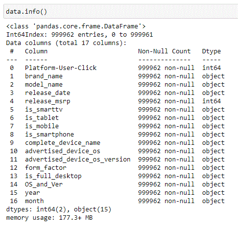
177 MB. Much better. This can be the basis for starting our research on a good ML model to understand a user’s propensity to click on our banner ad.
Machine Learning
If you have experience building regression models, you probably already noticed that we have
- quite a few variables and
- quite a few categorical variables
in our data.
Very generally speaking, data scientists do not love too many variables (they make building the model more complicated and time consuming) and they love categorical values even less (they tend not to play well with the mathematics powering (many) regression models). Understanding this is part of the foundation of data science and discussing it in detail would be beyond the scope of this article.
About removing unnecessary variables, a data scientist will try to discover which features (AKA independent variables) have limited or no influence on the dependent variable. Those that do (i.e. unimportant features) can be safely discarded from our model.
A column with the name of one of 50+1 US states would be a good example of categorical variables. Categorical variables with too many possible values create issues. To get an overview of the different approaches to turn categorical values into numbers before we fit our data, you can start here . Some methods (Label encoding) will turn values into numbers, with the side effect of introducing relations that are not in the original data. Other methods (One-Hot encoding) will introduce a new column for every categorical value, which may force your dataset to adopt a lot of new columns (i.e. features, i.e. independent variables) which complicates things.
We have this issue too, so we will need to remove unnecessary features first, then reduce the cardinality of certain categorical variables in order to apply One-Hot encoding, and after that we may find aspects of our data that allows us to reduce the number of features even more. Enough spoilers.
Certain features are safe to remove for sake of getting a simpler dataset without much analysis.
WURFL’s complete_device_name has lower cardinality than the User-Agent string, but still high enough that it won’t help in a (Machine Learning) regression model, so we can drop the column for now.

Columns such as is_smarttv,is_tablet,is_smartphone and is_full_desktop can be dropped as the information is captured by form_factor, which is the property that we will include in our model through dummy variables (i.e. One-Hot encoding).

As we have extracted year and month from the release_date column, we can remove it. ‘year’ and ‘month’ will do.

We have reduced the number of features, but as we prepare to perform one-hot encoding (dummy variables) on our categorical values, it is obvious that some of the features have a very long tail of possible values. We’ll need to reduce the “cardinality” of those variables, i.e. make sure that only the more significant values are accounted for.
Reducing Cardinality
Essentially, all categories that do not account for a certain percentage (or more) of the entries in the respective columns are consolidated under Other.
Let’s consider OS and Version for example. It’s a very long list going all the way into funky combinations that would hardly bear any real significance.
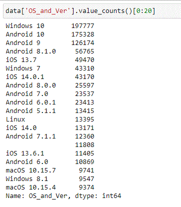
The following code will reduce the cardinality of brand_name, model_name and US_and_Ver by conflating all values that do not meet the 2% threshold representation in the dataset:

If you are not an experienced data scientist (also one that is versed in Python), the code above may appear daunting at first sight. Things should appear clearer if you are familiar with Numpy and will use a few minutes to familiarize yourself with np.where() and how it can selectively modify the values of cells in a matrix once you provide a suitable “mask”.
Here’s the result of our computation. Cardinality has been reduced to only account for the most popular entries:

We can also remove advertised_device_os and advertised_device_os_version at this point.

But we can do more. We have year and month. We can derive the age of the device (new device_age column) through some simple calculations (we used Pandas datetime, but a little lambda would have achieved the same).
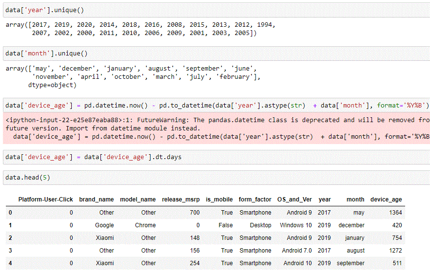
And of course we can also drop year and month at this point, which leaves us with a pretty clean dataset:

One-Hot Encoding
Time to turn our categorical data into sparse matrices of 0s and 1s.

df_coded.info()
<class 'pandas.core.frame.DataFrame'>
Int64Index: 999962 entries, 0 to 999961
Data columns (total 39 columns):
 #   Column                        Non-Null Count   Dtype
---  ------                        --------------   -----
 0   Platform-User-Click           999962 non-null  int64
 1   release_msrp                  999962 non-null  int64
 2   is_mobile                     999962 non-null  bool
 3   device_age                    999962 non-null  int64
 4   brand_name_Apple              999962 non-null  uint8
 5   brand_name_Google             999962 non-null  uint8
 6   brand_name_Huawei             999962 non-null  uint8
 7   brand_name_Microsoft          999962 non-null  uint8
 8   brand_name_Mozilla            999962 non-null  uint8
 9   brand_name_OPPO               999962 non-null  uint8
 10  brand_name_Other              999962 non-null  uint8
 11  brand_name_Samsung            999962 non-null  uint8
 12  brand_name_Vivo               999962 non-null  uint8
 13  brand_name_Xiaomi             999962 non-null  uint8
 14  model_name_Chrome             999962 non-null  uint8
 15  model_name_Edge               999962 non-null  uint8
 16  model_name_Firefox            999962 non-null  uint8
 17  model_name_Other              999962 non-null  uint8
 18  model_name_Safari             999962 non-null  uint8
 19  model_name_iPhone             999962 non-null  uint8
 20  form_factor_Desktop           999962 non-null  uint8
 21  form_factor_Feature Phone     999962 non-null  uint8
 22  form_factor_Other Mobile      999962 non-null  uint8
 23  form_factor_Other Non-Mobile  999962 non-null  uint8
 24  form_factor_Robot             999962 non-null  uint8
 25  form_factor_Smart-TV          999962 non-null  uint8
 26  form_factor_Smartphone        999962 non-null  uint8
 27  form_factor_Tablet            999962 non-null  uint8
 28  OS_and_Ver_Android 10         999962 non-null  uint8
 29  OS_and_Ver_Android 6.0.1      999962 non-null  uint8
 30  OS_and_Ver_Android 7.0        999962 non-null  uint8
 31  OS_and_Ver_Android 8.0.0      999962 non-null  uint8
 32  OS_and_Ver_Android 8.1.0      999962 non-null  uint8
 33  OS_and_Ver_Android 9          999962 non-null  uint8
 34  OS_and_Ver_Other              999962 non-null  uint8
 35  OS_and_Ver_Windows 10         999962 non-null  uint8
 36  OS_and_Ver_Windows 7          999962 non-null  uint8
 37  OS_and_Ver_iOS 13.7           999962 non-null  uint8
 38  OS_and_Ver_iOS 14.0.1         999962 non-null  uint8
dtypes: bool(1), int64(3), uint8(35)
memory usage: 64.8 MB
Lots of Dummy Variables, but still manageable. A look at our target (dependent) variable:

It is time to start thinking about training a model. As usual, we need to do the classic operations of getting a training set and test set.
Note: training set and test set are basic AI/ML concepts that you are expected to be familiar with already. If not, think of it this way: part of your data is used to build (train) the model, part of the data is used to measure how the model behaves (test). More modern and advanced approaches also call for a third set called the validation set to get reliable metrics on the model performance. Test and validation sets are confused at times. We only deal with training set and test set in our example.
In case of imbalanced data (our case), training and test set come with a caveat:
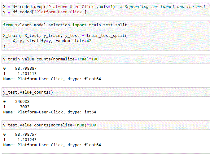
The caveat is the stratify=y parameter in our train_test_split(). This is normally not needed when building models and classifiers, as classes tend to be randomly distributed among test set and training set. As we explained earlier, though, we are in a special situation here. We are dealing with an imbalanced dataset, hence we need to give our “splitter” an additional directive to make sure that the few imbalanced data points are evenly distributed among test and training sets. value_counts() reveal that this has been the case (98.7 % vs 1.2% split in both cases).
Decision Tree Classifier
As every data scientist will know, we could start with a variety of strategies to build our classifier. A classifier is an algorithm (or function, or procedure) that, given some input data (features) will predict a result. For example, given a long list of test results and other data, a classifier may be able to predict with good accuracy whether the person has cancer or not.
In our case, we are looking for a classifier that, given an HTTP request, and after augmenting the data with WURFL capabilities, will guess whether the user will click on a banner ad.
Let’s start with a SkLearn DecisionTreeClassifier, taking all the default values for the hyperparameters (i.e. the parameters that we may tweak to tune the performance of a classifier).
Note: for the intuition behind Decision Trees, you can start here. As mentioned, we assume that you are familiar with basic ML concepts such as fitting your data to build the model.

The first model we built seems to have a fantastic “performance” as it provides 98% accuracy. Unfortunately things are not so good. We are dealing with an imbalanced dataset, which means that our classifier has taught itself that predicting 0 across the board (i.e. user will never click) is going to make its predictions right 98% of the times. This makes sense, but it does not help us much, though.
Yet, we are not going to discard our decision tree just yet, as it holds a barrage of useful information in store for us. Our data offers a lot of features. As you can imagine, they are probably not all equally important.
Note: If the concept of feature importance is already familiar to you, skip this note. If not, please pay attention as it is key to understanding the rest of the article. Imagine a dataset with a lot of columns that can be used to build a classifier (or a regressor for that matter). You may not be so surprised to discover that, say, the age of a patient correlates rather strongly to the possibility that they have cancer. On the other hand, it is very unlikely that the last 4 digits in a patient’s mobile phone number has any influence on their condition (or lack thereof). Age is an important feature in that case, while those last digits would carry no influence and one can safely ignore that bit of data in building their model: there would be no downsides. In this case, the first feature we described (the age) is important. The second not at all.
It should come as no surprise that data scientists have ways to measure the importance of the different features when building a model, and they can use that information to save time and money (models with less features are easier to build).
One cool feature of SkLearn Decision Tree is feature_importances_, i.e. the list of feature importances that will tell you which variables had the largest say in deciding how the tree ultimately took its decision.

Now, this is useful information! Thanks to the list of feature importances we can clearly see how two features, device age and price, overwhelmingly concur to predict whether a user will click or not. It’s always more likely that a user won’t click, but not all non-clicks are created equal. This is important information that will help us plan our next move.
But first, we can discard all features that have little importance. This will allow us to build our classifier in a matter of minutes, and not hours, even on a regular older laptop.

Random Forest Classifier
As usual, going into the details of how a random forest classifier is beyond the scope. Think of it as having many decision trees, and predictions are made based on the prevailing opinion of multiple trees. We are building a new classifier with the Random Forest this time because of one of its hyperparameters: class weight. Essentially, by tweaking class_weight, we can tell a RandomForestClassifier that it should give one of the classes (the 1 that represents the user click) way more importance than other classes (0 in our case). We expect this to bring forward the information that we are looking for about cases where users are more likely to click.

Accuracy has dropped to 50%. We are not surprised. The model is now predicting a lot of clicks, but when confronted with our test set, the prediction is way too optimistic. Let’s do some quick and dirty data visualization (DataViz) of our classifier.
First, we create lists of dummy data covering a wide array of price and device age combinations and capture the predictions in a Pandas dataframe.
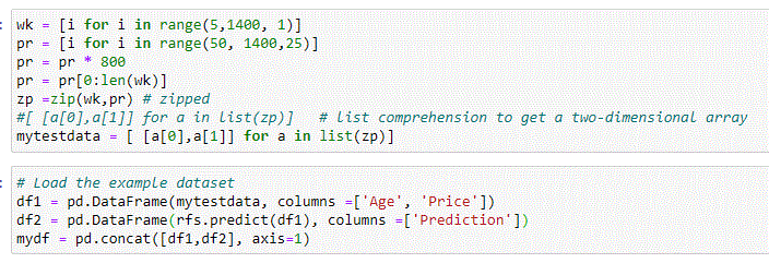
Let’s visualize:

Now we are talking. We can clearly see how users who own expensive devices that have been released two years earlier or less are somewhat more likely to click on a banner head. This is useful!
With this information, we have not quite reached our goal yet, but we are getting closer. If we wanted a model that helps us decide when to bid on an HTTP request (remember RTB), how do we get that? After all, we’ve tweaked our model to bring forward those occasions when users are more likely to click, but we still don’t have a measure of how likely a user is to actually click.
It turns out that our RandomForstClassifier has not run out of serendipity just yet, but in order to access that, we need to retrain our model. We won’t give 1’s more weight this time.

As expected, we get a very accurate (98%) but (apparently) useless classifier this time. For good measure, we confirm that the classifier predicts zeroes (no click) across the board.

Here comes the good stuff. The classifier has awesome metrics in store for us: predict_proba(). This property lets data scientists take a peek under the hood.
Note: Dear model, I am your creator and the one looking for an answer. I know that when I request a prediction you are going to tell me 0, but what’s the actual calculated probability that got you to give me that response? Is it 95%? Or 80%? Or simply 51%? Please tell me, because it matters a lot to me.
There’s a little bit of syntactic sugar to be aware of to access the good stuff (see first Jupyter cell below), but apart from that this is super useful. Our classifier knows exactly how likely it is that a user will click. And while a user is still unlikely to click, in some cases, they are more than 10% likely to click on an ad (see below).
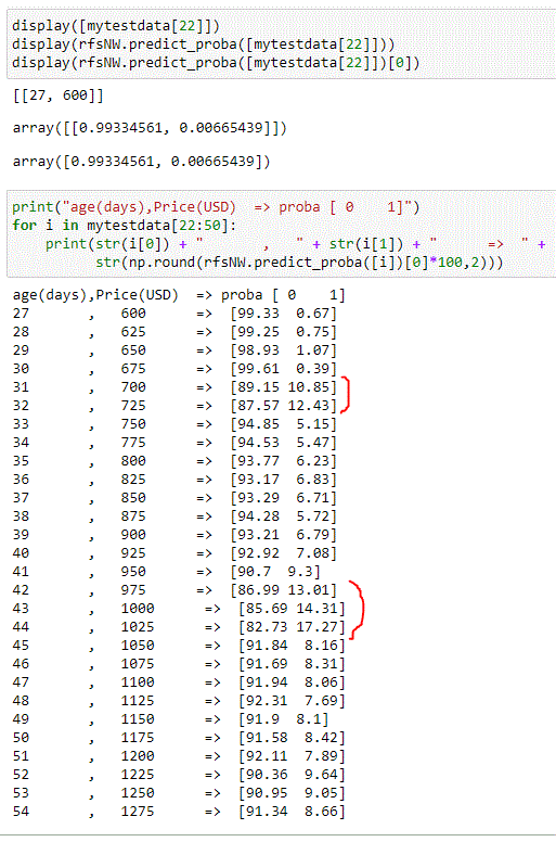
The second figure provides an estimate of the probability that a user clicks on a banner based on their device. While we highlighted figures above 10% probability, one can decide that they are interested in events where that threshold is 5% or above, or 8% or above. In short, this is the model we were looking for!
Given an HTTP request, thanks to WURFL we can calculate in real-time the probability that a user will click on our banner ad and take a decision based on that information. In fact, this model has a further advantage: it does not depend on the User-Agent string directly. Once a device age and price are determined through WURFL, the model will do the rest and is likely to perform similarly as new devices hit the market and as existing devices get older (and as such their cost decreases).
Arguably, the model we have obtained is good enough for production. In a real scenario, once this model is in place, you can use any WURFL API for any supported language/platform to obtain a device age and price in real-time. Feeding those figures to our model will provide an estimate of how likely a user is to click. You can use that figure to take a decision.
Conclusions
This was one of our longest blogs ever, but we had a lot of ground to cover. AI/ML is a vast and complex subject. Experienced data scientists should feel right at home with what we wrote and may even find this article easy reading. Newbies will find it more complex because of the sheer amount of new concepts. Hopefully, we managed to convey the gist of what was going on and the references to each subject did the rest. In the end, this might be an introduction to the subject for some. Hopefully, once everyone is on the same page, they recognize the additional value that WURFL can bring to the analysis of logs and user behavior.
Resources
You can find the Jupiter Notebooks that we used for the article here. The example has been split in three separate notebooks for ease of use:
- Notebooks: https://github.com/WURFL/machine-learning/
- Dataset (1 million HTTP requests in JSON format): https://github.com/WURFL/machine-learning/blob/main/feb_2021_article/data.json.gz
While we provided the data files for educational purposes, the notebook that extracts device information will require use of the Python API for WURFL and a custom version of the WURFL data that includes the device price at the time of release. These tools are licensed commercially by ScientiaMobile.
For licensing and trials, you can visit the ScientiaMobile license inquiry page and select the Device Detection use case.


